Category: IT

  • Building Elmer FEM with 3D AMR on Ubuntu 24 LTS – A Practical Guide

    At TSG USA Inc., our mechanical design team regularly holds study sessions on finite element analysis (FEA). Commercial FEA software is often prohibitively expensive for small companies, especially for training purposes. For this reason, we decided to adopt Elmer, an open-source FEA software package, as our learning platform.

    Background

    Since all team members use Windows PCs, we initially installed Elmer using precompiled binaries. However, we encountered a key limitation:

    The Windows binary does not include 3D Adaptive Mesh Refinement (AMR).

    Without AMR, it is difficult to evaluate mesh quality and ensure reliable simulation results. Therefore, we decided to build Elmer from source with:

    • 3D AMR support
    • ElmerGUI
    • Parallel computation (OpenMP & MPI)

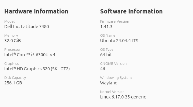
    We used Ubuntu 24 LTS installed natively on standalone PCs, since Linux-based build instructions were available and compatible machines were readily accessible.

    Specification of the Linux PC that we used.

    We also built ParaView from source, because the packaged version produced errors when opening Elmer output .vtu files.

    Procedures written in this article follow these references:

    Preparation

    To make the installation accessible to all users, we installed everything under /usr/local/ directory.

    Installing required packages

    First, we installed required packages using apt as follows:

    sudo apt install git cmake build-essential gfortran \
         libopenmpi-dev libblas-dev liblapack-dev
    sudo apt install libqwt-qt5-dev
    sudo apt install libqt5opengl5-dev
    sudo apt install qtscript5-dev
    sudo apt install libqt5svg5-dev
    sudo apt install libmpich-dev libnetcdff-dev \ 
         libmetis-dev libparmetis-dev libmumps-dev \
         netcdf-bin
    sudo apt install lua5.3

    Building Elmer Dependencies

    We then built and installed required libraries: CSA, NN, MMG, and parMMG. We used the following compiler options throughout.

    export CFLAGS="-fPIC  -O2"
    export CC=gcc

    Building CSA

    git clone https://github.com/sakov/csa-c
    cd csa-c/csa
    ./configure --prefix="/usr/local"
    make
    sudo make install
    cd ../..

    Building NN (with modification)

    git clone https://github.com/sakov/nn-c
    cd nn-c/nn/
    ./configure --prefix="/usr/local"

    We edited one line in Makefile:

    CFLAGS_TRIANGLE = -O2 -w -ffloat-store

    as:

    CFLAGS_TRIANGLE = -O2 -w -ffloat-store -fPIC

    Then executed:

    make
    sudo make install
    cd ../..

    Building MMG

    git clone https://github.com/MmgTools/mmg.git
    cd mmg
    git checkout 4d8232c
    mkdir build
    cd build
    cmake -D CMAKE_INSTALL_PREFIX="/usr/local" \
          -D CMAKE_BUILD_TYPE=RelWithDebInfo \
          -D BUILD_SHARED_LIBS:BOOL=TRUE \
          -D MMG_INSTALL_PRIVATE_HEADERS=ON \
          -D CMAKE_C_FLAGS="-fPIC  -g" \
          -D CMAKE_CXX_FLAGS="-fPIC -std=c++11 -g" ..
    make
    sudo make install
    cd ../..

    Building parMMG

    git clone https://github.com/MmgTools/parmmg
    cd parmmg
    git checkout cd8a6e3
    mkdir build
    cd build
    cmake -D CMAKE_INSTALL_PREFIX="/usr/local" \
          -D CMAKE_BUILD_TYPE=RelWithDebInfo \
          -D BUILD_SHARED_LIBS:BOOL=TRUE \
          -D DOWNLOAD_MMG=OFF \
          -D MMG_DIR="/opt/elmer/elmerdependencies" ..
    make
    sudo make install
    cd ../..

    Building Elmer FEM

    After building and installing the dependencies as shown above, we proceeded to building and installing Elmer.

    git clone https://github.com/ElmerCSC/elmerfem.git
    cd elmerfem
    git submodule update --init
    git checkout 4f69f075e
    cd ..
    
    mkdir build
    cd build
    
    cmake -DCMAKE_INSTALL_PREFIX="/usr/local" \
          -DWITH_MPI=TRUE \
          -DWITH_LUA=TRUE \
          -DWITH_OpenMP=TRUE \
          -DWITH_Mumps=TRUE \
          -DWITH_Hypre=TRUE \
          -DHypre_INCLUDE_DIR="/usr/include/hypre" \
          -DWITH_Trilinos=FALSE \
          -DWITH_ElmerIce=FALSE \
          -DWITH_Zoltan=TRUE \
          -DWITH_MMG=TRUE \
          -DWITH_PARMMG=TRUE \
          -DWITH_NETCDF=TRUE \
          -DWITH_ScatteredDataInterpolator=TRUE \
          -DWITH_ELMERGUI=TRUE \
          -DWITH_QT5=TRUE \
          -DWITH_QWT=TRUE \
          -DWITH_MATC=TRUE \
          -DWITH_PYTHONQT=FALSE \
          ../elmerfem
    
    make
    ctest
    sudo make install

    Note that ctest is optional above.

    In the process above we used the following git commit as those were already tried and worked in the following reference. Elmerをコンパイルするシェルスクリプト #WSL2 – Qiita:

    • MMG commit: 4d8232c
    • parMMG commit: cd8a6e3
    • Elmer FEM commit: 4f69f075e

    Building ParaView from Source

    We encountered errors when opening Elmer output .vtu files with the packaged ParaView, so we built it manually. We referred to the following page. Documentation/dev/build.md · master · ParaView / ParaView · GitLab

    Installing dependencies

    sudo apt install libgl1-mesa-dev libxt-dev \
         libqt5x11extras5-dev libqt5help5 \
         qttools5-dev qtxmlpatterns5-dev-tools \
         python3-dev python3-numpy libtbb-dev \
         ninja-build qtbase5-dev qtchooser qt5-qmake \ 
         qtbase5-dev-tools

    Building ParaView

    git clone https://gitlab.kitware.com/paraview/paraview.git
    mkdir paraview_build
    cd paraview
    git submodule update --init --recursive
    cd ../paraview_build
    
    cmake -GNinja \
          -DPARAVIEW_USE_PYTHON=ON \
          -DPARAVIEW_USE_MPI=ON \
          -DVTK_SMP_IMPLEMENTATION_TYPE=TBB \
          -DCMAKE_BUILD_TYPE=Release \
          -DCMAKE_INSTALL_PREFIX="/usr/local" \
          ../paraview
    
    ninja
    sudo cmake -P cmake_install.cmake

    Testing 3D AMR

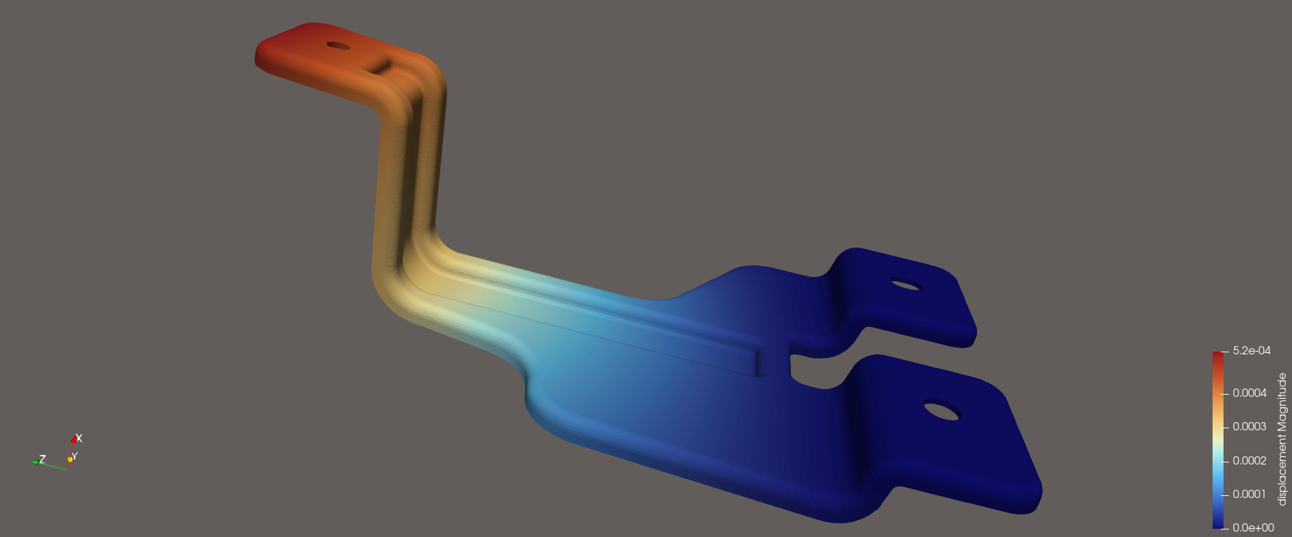
    We performed a linear elasticity analysis with AMR enabled. We used a training 3D model created by our mechanical design team. The .sif file used to run the Elmer simulation was as follows:

    Header
      CHECK KEYWORDS Warn
      Mesh DB "." "."
      Include Path ""
      Results Directory ""
    End
    
    Simulation
    ! Importance level of output message 
    ! (1 being most important)
    ! The larger the number is, 
    ! the more verbose output messages become.
      Max Output Level = 6
      Coordinate System = Cartesian
      Coordinate Mapping(3) = 1 2 3
      Simulation Type = Steady state
      Steady State Max Iterations = 6
      Output Intervals(1) = 1
      Solver Input File = bracket.sif
      Post File = bracket.vtu
      Output File = bracket.result
      Convergence Monitor = True
    End
    
    Constants
      Gravity(4) = 0 -1 0 9.82
      Stefan Boltzmann = 5.670374419e-08
      Permittivity of Vacuum = 8.85418781e-12
      Permeability of Vacuum = 1.25663706e-6
      Boltzmann Constant = 1.380649e-23
      Unit Charge = 1.6021766e-19
    End
    
    Body 1
      Target Bodies(1) = 1
      Name = "Body 1"
      Equation = 1
      Material = 1
    End
    
    Solver 1
      Equation = Linear elasticity
      Calculate Stresses = True
      Procedure = "StressSolve" "StressSolver"
      Exec Solver = Always
      Stabilize = True
      Optimize Bandwidth = True
      Steady State Convergence Tolerance = 1.0e-2
      Nonlinear System Convergence Tolerance = 1.0e-7
      Nonlinear System Max Iterations = 20
      Nonlinear System Newton After Iterations = 3
      Nonlinear System Newton After Tolerance = 1.0e-3
      Nonlinear System Relaxation Factor = 1
      Linear System Solver = Direct
      Linear System Direct Method = mumps 
      mumps percentage increase working space = 80
      Displace Mesh = True
      Adaptive Mesh Refinement = True
      Adaptive Remesh = True
      adaptive remesh use mmg = True
      Adaptive Coarsening = True
      Adaptive Save Mesh = True
      Adaptive Min H = 0.00018
      Adaptive Max H = 0.0018
      Adaptive Error Limit = 1.3e-4
    ! Pre smoothing averages nodal error estimates before 
    ! driving adaptive mesh refinement.
    ! Pre smoothing prevents the mesh from over-
    ! refinement.
      Adaptive Pre Smoothing = 4
      Adaptive Error Histogram = True
    End
    
    Equation 1
      Name = "Equation 1"
      Active Solvers(1) = 1
    End
    
    Material 1
      Name = "Structural Steel"
      Poisson ratio = 0.305
      Heat Capacity = 976.0
      Youngs modulus = 210.0e9
      Heat Conductivity = 37.2
      Sound speed = 5100.0
      Density = 7850.0
      Heat expansion Coefficient = 12.0e-6
    End
    
    Boundary Condition 1
      Target Boundaries(1) = 145 
      Name = "BoundaryCondition 1"
      Displacement 2 = 0
      Displacement 1 = 0
      Displacement 3 = 0
    End
    
    Boundary Condition 2
      Target Boundaries(1) = 216 
      Name = "BoundaryCondition 2"
      Displacement 3 = 0
      Displacement 2 = 0
      Displacement 1 = 0
    End
    
    Boundary Condition 3
      Target Boundaries(1) = 288 
      Name = "Press down"
      Normal Force = -10600.61
    End

    We named this .sif file as “bracket.sif”. To run the simulation with OpenMP, we used the following command:

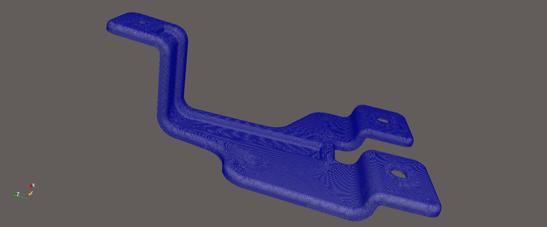
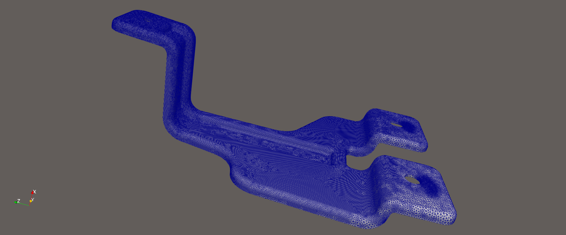
    OMP_NUM_THREADS=4 ElmerSolver bracket.sif

    Note that our laptop had 4 cores in its CPU, thus the number of the OpenMP threads was set at 4. The simulation converged after five remeshing iterations. The meshes before and after AMR are shown in the figures below. These figures are created using ParaView that we built from its source and installed.

    The initial mesh is relatively uniform across the entire geometry, without considering stress or displacement distribution.
    After applying AMR, the mesh density automatically adapts. Fine mesh in regions where displacement is large. Coarser mesh in regions where displacement is small.
    The high-displacement regions correspond to areas with finer mesh after AMR.

    AMR Convergence Study

    We varied the parameter Adoptive Error Limit in our .sif file and compared results of Max Displacement, Max VonMises, Max Error and Error Estimate obtained from each simulation.

    Adaptive Error LimitMax DisplacementMax VonMisesMax ErrorError Estimate
    1.0e-25.7e-46.1e73.28e-42.41e-5
    3.0e-45.7e-46.1e72.40e-42.37e-5
    2.0e-46.0e-47.5e71.50e-41.23e-5
    1.3e-46.2e-47.7e77.90e-56.50e-5

    First, we set a relaxed Adaptive Error Limit, i.e. 1.0e-2, and executed a simulation. Then, for the second simulation, we set slightly tighter Adaptive Error Limit, i.e. 3.0e-4, than the Max Error obtained from the first simulation, i.e. 3.28e-4. We repeated this process and observed how the results of Max Displacement and Max VonMises vary.

    Remaining Challenge

    While testing ElmerGUI, we noticed that STEP files and STL files could not be opened. After some studies, we learned that this issue was caused by missing linkage with OpenCASCADE (OCC) to ElmerGUI. For this reason, we installed OpenCASCADE using apt:

    sudo apt install -y xfonts-scalable \
         libocct-data-exchange-dev \
         libocct-draw-dev \
         libocct-foundation-dev \
         libocct-modeling-algorithms-dev \
         libocct-modeling-data-dev \
         libocct-ocaf-dev \
         libocct-visualization-dev

    Then we attempted to rebuild ElmerGUI with the flag:

    -DWITH_OCC:BOOL=TRUE

    However, this resulted in CMake errors and the build did not succeed. Thus, our next goal is to properly link OpenCASCADE to ElmerGUI and to enable STEP/STL import in ElmerGUI.

    Conclusion

    By building Elmer and ParaView from source, we achieved 3D AMR functionality and reliable visualization. This setup provides a powerful and cost-effective FEA learning environment for our team. We hope this guide will be helpful to others working in similar situations.

  • Predicting the Future of IoT Data: A Practical Guide to Machine Learning

    Predicting the Future of IoT Data: A Practical Guide to Machine Learning

    In many businesses today, installing IoT devices and collecting sensor data has become standard practice. Your organization might be gathering thousands of data points—such as voltage, temperature, or load—every single day. While visualizing this historical or real-time data on a dashboard is a valuable first step, it only tells you what is happening right now.

    But what if your system could tell you exactly how many hours of operational life your device has left before it stops?

    Transitioning from “current status monitoring” to “future prediction” might sound like a complex task reserved for enterprises with massive data science teams. You may think, “Building AI models is too expensive and requires deep mathematical expertise.” However, it is entirely possible to build a custom predictive architecture tailored to your specific hardware. By integrating BigQuery, Vertex AI, and AutoML, you can transform scattered IoT sensor data into a highly accurate, real-time forecasting engine.

    The Three Technologies for Prediction

    To make your data predictable, you need a system that can securely store historical data, perform feature engineering to find hidden correlations, and process real-time inference requests. Here is how this architecture functions:

    1. BigQuery: The Data Ingestion and Preprocessing Foundation

    Before you can predict the future, you must establish a baseline from the past. Every second of sensor data your devices generate is securely ingested into BigQuery. As a highly scalable data warehouse, BigQuery stores tens of thousands of historical operation and discharge logs. It acts as the primary data preprocessing environment where raw data is cleaned and structured before being passed to the machine learning engine.

    2. Vertex AI & AutoML: Automated Feature Engineering and Regression

    Prediction models cannot be built simply by plotting current voltage against time. To predict remaining hardware life accurately, we must analyze historical discharge cycles and identify multi-variable correlations. Inside Vertex AI, AutoML handles this complex process. Rather than manually testing algorithms, AutoML automatically performs feature engineering and selects the optimal regression model based on your BigQuery dataset. It autonomously maps specific voltage drop patterns to their corresponding remaining operational timelines.

    3. Real-Time Inference Application

    Once AutoML finishes building the model, it is deployed directly within BigQuery using ML.PREDICT. This means your frontend applications can execute predictions using standard SQL queries without needing a separate, dedicated ML hosting server. For instance, in our recent setup, a custom dashboard sends current voltage readings to a backend API. Within milliseconds, the API queries the trained model and returns the predicted remaining operational minutes to the user.

    Predicted Remaining Life  Demo Page

    Moving from Reactive to Predictive

    You don’t need to write complex algorithms from scratch to benefit from machine learning. By utilizing BigQuery to structure historical data and allowing Vertex AI and AutoML to discover predictive rules autonomously, your business can shift from merely reacting to real-time IoT alerts to proactively planning maintenance and optimizing hardware lifecycles.

    At TSG USA Inc., we specialize in turning raw IoT data into actionable intelligence. Whether you need Vertex AI integration or comprehensive Google Cloud architecture, our team is ready to build your next predictive system. Contact us today to get started.

  • Designing a Custom Database: A Practical Guide for Small Businesses

    In small businesses, it is often the case that various data used for administrative tasks are stored in scattered Excel files. While Excel is a great tool for analyzing numerical data, it is not well-suited for searching, aggregating, bulk updating non-numerical data, or joining data from multiple files. One simple solution to this “Excel pain” is to use relational databases instead.

    You may think, “Licenses for database software are expensive and only for big companies,” or “We can’t hire people to build and operate databases because it’s complicated and requires special expertise.” However, we can show you that it’s not so difficult to build a small custom database tailored to your needs. Even better, there are open-source solutions to host your database.

    What You Need Before Getting Started

    Before you get your hands dirty building a database, you need the following:

    • A clear objective for your database
    • An understanding of (or curiosity to learn) the first, second, and third normal forms of database design
    • The ability to draw an Entity Relationship Diagram (ERD)

    The second and third items may sound intimidating if you’ve never heard of them. But don’t worry—you don’t need to dive deep. A surface-level understanding is more than enough, and no advanced math is required.

    Understanding Relational Databases

    Relational databases are composed of tables organized for specific purposes. Let’s assume we want to build a database to store information on insurance enrollment in your company. We want to be able to look up which employees are enrolled in which insurance policies—and vice versa. To begin, we’ll create two tables: one for employees and one for insurance policies.

    Each row in a table represents an entity (e.g., an employee or a policy), and each column represents an attribute (e.g., first name or premium). For example, the employee table includes attributes such as first name, last name, and date hired. The insurance policy table includes attributes such as policy name, enrollee, premium, and dependent enrollment status (e.g., “employee only”, “employee and spouse”, or “family”).

    First Normal Form (1NF)

    According to the first normal form, every row in a table must be unique. Let’s consider our employee table. If the company has two employees named Ichiro Suzuki who were both hired on the same day, the table would contain duplicate rows—violating 1NF.

    The solution is to add an identification number to each table to uniquely identify each row. This is known as a primary key (PK). In our case, we add employee_id and insurance_policy_id as the primary keys of the employee and insurance policy tables, respectively.

    Second Normal Form (2NF)

    The second normal form requires that each non-primary-key attribute in a table must be fully dependent on the primary key. Our employee table now meets this requirement because all attributes (first_name, last_name, date_hired) depend solely on employee_id.

    However, in the insurance policy table, attributes like enrollee, dependent_enrollment, and premium are not determined solely by insurance_policy_id, since each policy can have multiple enrollees. These attributes depend on the relationship between employees and policies.

    To address this, we create a new table, insurance_policy_enrollment, with employee_id and insurance_policy_id as foreign keys (FKs). This table represents who is enrolled in which policy.

    Next, we move the dependent_enrollment and premium attributes into the insurance_policy_enrollment table, because they depend on both employee_id and insurance_policy_id.

    Third Normal Form (3NF)

    The third normal form requires that every attribute must depend only on the primary key—not on another non-key attribute.

    Our employee table already satisfies this condition. Now, let’s check the insurance_policy_enrollment table. Here, the combination of employee_id and insurance_policy_id is the primary key. But attributes like dependent_enrollment and premium are not strictly dependent on this combination. For example, if an employee has a child, their dependent enrollment status might change, which in turn might affect the premium.

    To normalize further, we:

    1. Create a new table, dependent_enrollment_type, where dependent_enrollment is a key.
    2. Link this to the insurance_policy_enrollment table via a foreign key.
    3. Create another table, insurance_policy_dependent_enrollment, to map the relationship between insurance policy and dependent enrollment type with associated premiums.

    Now all tables meet the requirements of the third normal form.

    Final Touch: Add Integer Primary Keys

    As a best practice, each table should have an integer primary key for better performance and easier management, especially when using database software such as MySQL or PostgreSQL.

    Wrapping Up

    Our objective was to build a database that can help you identify:

    • Which employees are enrolled in which insurance policies
    • Which insurance policies are enrolled by which employees

    This is accomplished through queries that join the employee, insurance_policy_enrollment, and insurance_policy tables.

    When renewing a contract with your insurance provider, premiums may change. Instead of manually updating every row in a spreadsheet, you only need to update the insurance_policy_dependent_enrollment table—reducing the risk of human error.

    Best of all, free and open-source tools like MySQL and PostgreSQL can host your database effortlessly.

    Let’s Chat!

    Are you interested in building custom databases for your organization but not sure where to start? Let’s talk! Feel free to reach out to us on our LinkedIn page. We’d love to learn about your needs and help you find a solution.